Performance theory: latency, throughput, bandwidth, parallelism vs concurrency & Little's Law
Understand latency(P50/P95/P99/P999), throughput, bandwidth, load, capacity, utilization, service time, response time, queueing, concurrency vs parallelism, percentiles, tail latency & Little's Law

Latency and Throughput
These two metrics are often confused. They measure different things.
Latency is the time between sending a request and receiving a response. It is measured in time units: milliseconds, microseconds, seconds. Low latency means the system responds quickly.
Throughput is the number of requests a system can process per unit of time. It is measured in operations per second: QPS (queries per second), RPS (requests per second), TPS (transactions per second). High throughput means the system does a lot of work.
The relationship is not fixed. A system can have low latency and low throughput. It can have high latency and high throughput. Batch processing systems often have high latency (minutes per job) and very high throughput (millions of records per second). Real-time APIs have low latency (tens of milliseconds) and moderate throughput.
The confusion arises because increasing throughput often increases latency. When a system handles more requests simultaneously, those requests wait in queues. Queueing adds latency.
Bandwidth
Bandwidth is the maximum amount of data that can be transferred per unit of time. It is measured in bits or bytes per second: Mbps, Gbps, MB/s.
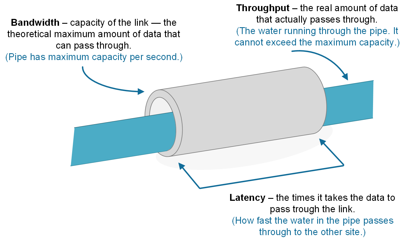
Bandwidth and throughput are related but distinct. Bandwidth is a capacity limit. Throughput is actual usage. A 1 Gbps network link has 1 Gbps of bandwidth. If you send 200 Mbps through it, your throughput is 200 Mbps and your bandwidth is 1 Gbps. If you try to send 2 Gbps, your throughput will cap at 1 Gbps and packets will be dropped or delayed.
For system design, bandwidth matters when moving large amounts of data. Streaming video, transferring database backups, and serving large files are bandwidth-bound. API calls with small payloads are rarely bandwidth-bound; they are latency-bound or CPU-bound.
This diagram illustrates the conceptual difference between the three metrics
Load, Capacity, and Utilization
These three concepts form the foundation of capacity planning.
Load is the rate at which work arrives at the system. It is measured in requests per second. It is often denoted by the Greek letter lambda (λ).
Capacity is the maximum rate at which the system can process work. It is measured in the same units as load: requests per second. It is often denoted by mu (μ).
Utilization is the fraction of capacity being used. It is calculated as:
A system with a capacity of 100 requests per second receiving 70 requests per second has 70% utilization. A system receiving 120 requests per second has 120% utilization. It is overloaded.
The critical insight is that utilization cannot exceed 100% in steady state. When it approaches 100%, queueing delays grow rapidly. A system at 90% utilization has significantly higher latency than the same system at 50% utilization, even though both are processing the same number of requests per second. This is why production systems aim to keep utilization below 70-80%. The remaining capacity is headroom for traffic spikes.
Service Time and Response Time
These two are often used interchangeably. They should not be.
Service time is the time the system actively spends processing a request. It includes CPU time, disk I/O time, and any computation. It does not include waiting.
Response time is the total time from request arrival to response departure. It includes service time plus all waiting time.
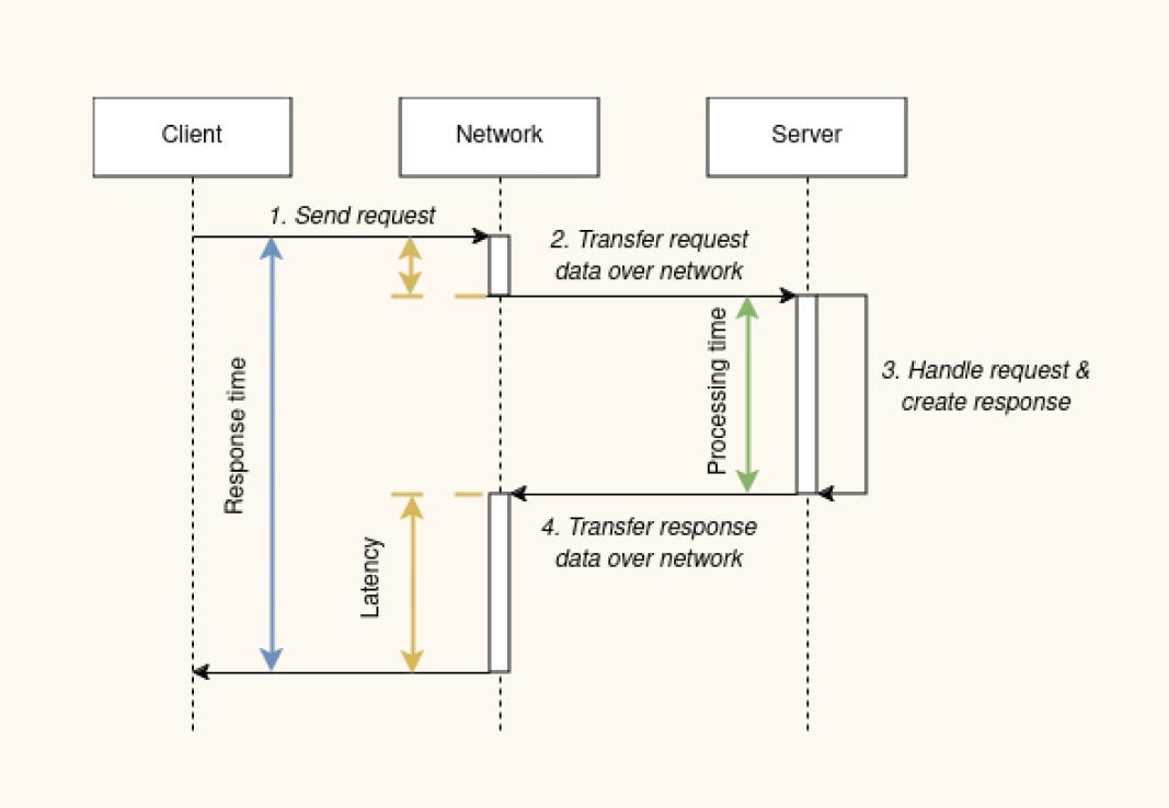
The distinction matters because it tells you where to look for problems. If response time is high but service time is low, the request spent most of its life waiting. The bottleneck is queueing somewhere: a saturated CPU scheduler, a full connection pool, a lock contention. If service time is high, the work itself is slow. The fix is optimization or vertical scaling.
Without measuring both, you cannot tell the difference. Most monitoring systems measure response time. Few measure service time. This is a common blind spot.
Queueing and Little’s Law
Queueing is the reason systems slow down under load. When requests arrive faster than they can be processed, they form a queue. The queue adds waiting time to every request.
Little’s Law (L = lambda * reponse time(avg)) is the fundamental relationship that governs queueing systems:
This law holds for any stable system, regardless of the distribution of arrivals or service times. It is one of the few universal truths in performance analysis.
For example, if 50 requests arrive per second (λ = 50) and each request takes 0.1 seconds on average (W = 0.1), then the average number of requests in the system is L = 50 × 0.1 = 5. Five requests are either being processed or waiting.
For a simple single-server queue (M/M/1 model), the average queueing time can be calculated:
This formula reveals why utilization matters so much. At 50% utilization, queue time equals service time. Response time is twice service time. At 80% utilization, queue time is four times service time. Response time is five times service time. At 90% utilization, queue time is nine times service time. Response time is ten times service time. Latency explodes long before the system reaches 100% utilization.
Concurrency vs Parallelism
These terms are often used as synonyms. They are not the same. The distinction matters because it determines how you structure your code and how you reason about throughput.
Concurrency
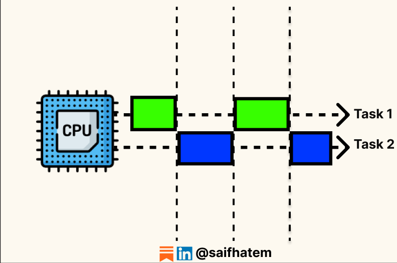
Concurrency means a system makes progress on multiple tasks during the same time period, but not necessarily at the same instant. On a single CPU core, concurrency is achieved by rapidly switching between tasks. The CPU works on task A for a few milliseconds, saves its state, switches to task B, then to task C, and back to task A. The switching happens so quickly that tasks appear to run simultaneously.
The primary goal of concurrency is to maximize CPU utilization by minimizing idle time. When one thread waits for I/O, a database query, or a network response, the CPU can switch to another thread and do useful work instead of sitting idle.
How it works: The CPU performs context switching. It saves the current task’s state (program counter, registers) into memory, then loads the saved state of the next task and resumes execution. Context switching has overhead. Each switch consumes time and flushes CPU caches. Excessive switching degrades performance.
Java example — concurrent task execution:
public class ConcurrencyExample {
    public static void main(String[] args) {
        Thread taskA = new Thread(() -> {
            for (int i = 1; i <= 3; i++) {
                System.out.println(”Task A - Step “ + i);
                try { Thread.sleep(100); } catch (InterruptedException e) {}
            }
        });

        Thread taskB = new Thread(() -> {
            for (int i = 1; i <= 3; i++) {
                System.out.println(”Task B - Step “ + i);
                try { Thread.sleep(100); } catch (InterruptedException e) {}
            }
        });

        taskA.start();
        taskB.start();
    }
}
Sample output (interleaved):
text
Task A - Step 1
Task B - Step 1
Task A - Step 2
Task B - Step 2
Task A - Step 3
Task B - Step 3
The tasks do not run simultaneously. The CPU interleaves them. On a single-core machine, only one thread executes at any given instant. On a multi-core machine, threads may also run in parallel, but the code above does not guarantee parallelism.
Real-world examples of concurrency:
Web browsers rendering a page while downloading images and responding to scroll events
Web servers (Apache, Nginx) handling thousands of client connections with fewer threads than connections
Chat applications processing incoming messages while updating the UI
Video games rendering graphics, processing input, and playing audio in overlapping time windows
Parallelism
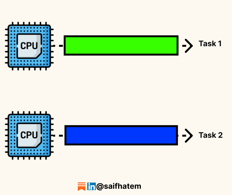
Parallelism means multiple tasks execute at exactly the same instant. This requires multiple CPU cores or multiple machines. A task is divided into smaller independent subtasks, and each subtask runs simultaneously on a separate processing unit.
The primary goal of parallelism is to increase throughput by doing more work per unit of time. If a task takes 10 seconds on one core, splitting it into 10 equal subtasks across 10 cores can theoretically complete in 1 second.
How it works: The problem is divided into independent subtasks. Each subtask is assigned to a separate core. All cores execute simultaneously. Results are combined at the end.
Java example — parallel computation using ForkJoinPool:
import java.util.concurrent.RecursiveTask;
import java.util.concurrent.ForkJoinPool;

public class ParallelismExample extends RecursiveTask<Long> {
    private static final int THRESHOLD = 10_000;
    private final int[] array;
    private final int start;
    private final int end;

    public ParallelismExample(int[] array, int start, int end) {
        this.array = array;
        this.start = start;
        this.end = end;
    }

    @Override
    protected Long compute() {
        int length = end - start;
        if (length <= THRESHOLD) {
            // Sequential computation for small chunks
            long sum = 0;
            for (int i = start; i < end; i++) {
                sum += array[i];
            }
            return sum;
        } else {
            // Split and run in parallel
            int mid = start + length / 2;
            ParallelismExample left = new ParallelismExample(array, start, mid);
            ParallelismExample right = new ParallelismExample(array, mid, end);

            left.fork();  // Run left task asynchronously
            long rightResult = right.compute();  // Compute right task
            long leftResult = left.join();       // Wait for left task

            return leftResult + rightResult;
        }
    }

    public static void main(String[] args) {
        int[] array = new int[100_000];
        // Initialize array...

        ForkJoinPool pool = new ForkJoinPool();
        long sum = pool.invoke(new ParallelismExample(array, 0, array.length));
        System.out.println(”Sum: “ + sum);
    }
}
Real-world examples of parallelism:
Machine learning training: datasets divided into batches, processed simultaneously across multiple GPUs
Video rendering: each frame rendered independently on a different core
Web crawlers: URL list split into chunks, fetched in parallel from multiple websites
Big data frameworks (Apache Spark): large datasets distributed across clusters for simultaneous processing
Scientific simulations: weather modeling, molecular dynamics divided across thousands of cores
The Four Combinations
A system can be concurrent, parallel, both, or neither.
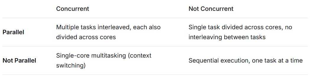
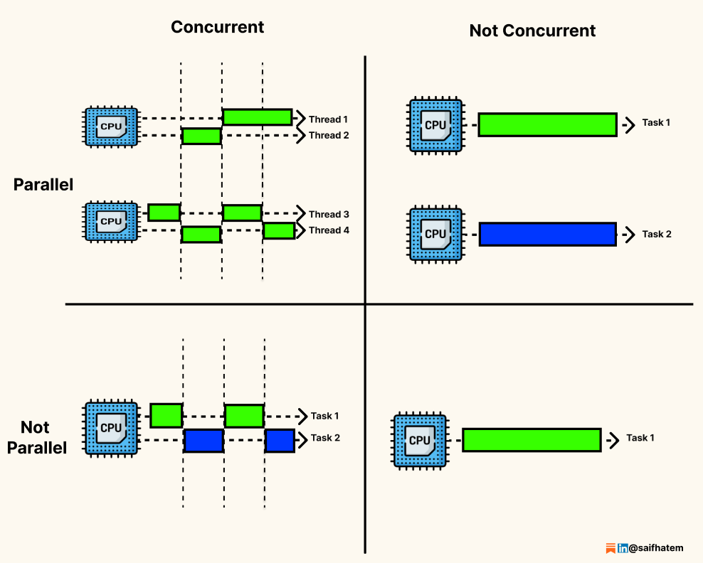
Concurrent, not parallel: A single-core CPU running a web browser. The browser handles network requests, rendering, and user input by switching rapidly between tasks. Only one task executes at any instant, but progress is made on all of them.
Parallel, not concurrent: A video rendering job divided into 8 frames, processed on 8 cores simultaneously. The system works on only one logical task (rendering the video), but that task is broken into parallel subtasks.
Neither concurrent nor parallel: A batch script that reads a file, processes it line by line, and writes output. One thing happens at a time. No overlapping progress. No simultaneous execution.
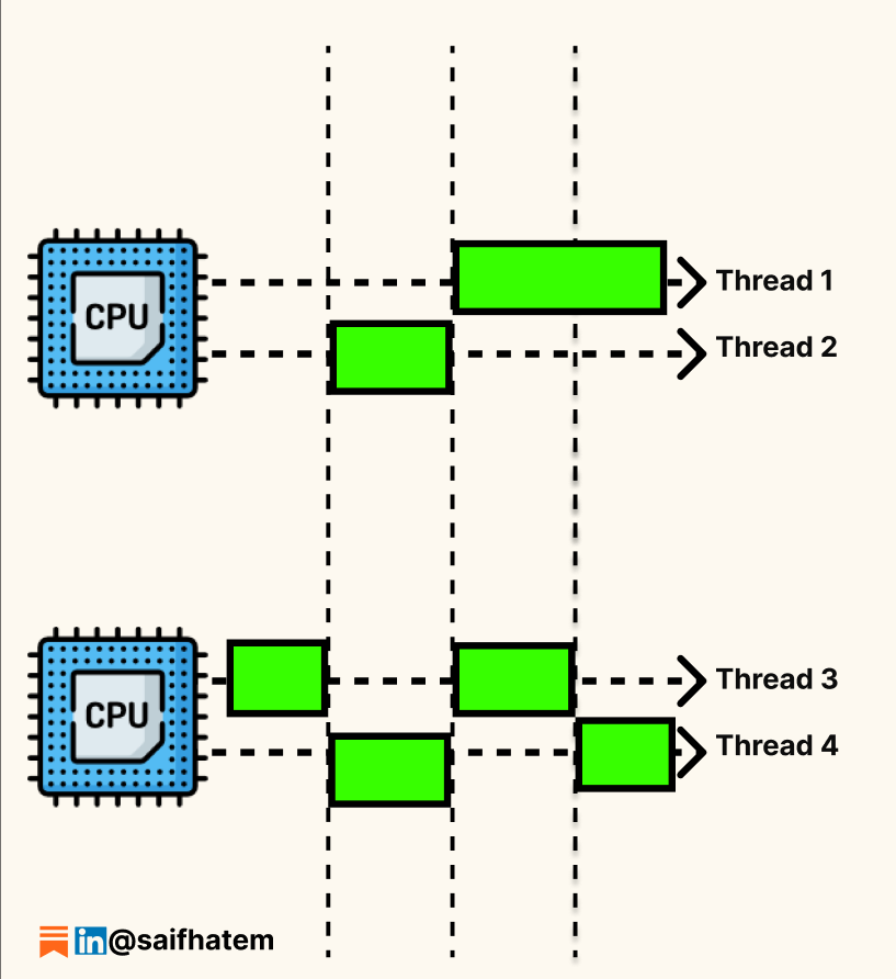
Concurrent and parallel: A multi-core web server handling thousands of client connections. Each connection is managed concurrently via threads or async I/O. Within each connection, work may also be parallelized across cores. This is the most common pattern in modern high-performance systems. The diagram below illustrates this
The Practical Takeaway
Concurrency is about structure. It is a way to write code that deals with multiple things at once without blocking. Parallelism is about execution. It is a way to use hardware to do more work per second.
You need concurrency when your system waits for I/O. You need parallelism when your system does heavy computation. Many systems need both. The Java examples above show the difference: threads for concurrency, ForkJoinPool for parallelism.
In system design interviews, using these terms correctly signals that you understand the difference. Describing a web server as “parallel” is wrong. It is concurrent. Describing a batch processing job as “concurrent” misses the point. It is parallel. Precision matters.
Percentiles and Tail Latency
Most people think about latency in terms of averages. The average is the sum of all request latencies divided by the number of requests. This single number hides almost everything that matters.
Why Average Latency Is Misleading
Take 100 API requests. 99 of them finish in 10 milliseconds. 1 request takes 10 seconds (10,000 milliseconds).
The average latency is:
text
(99 × 10ms + 1 × 10,000ms) / 100 = 10,990ms / 100 = 109.9msThe average is about 110 milliseconds. That looks excellent. But one out of every hundred users just waited ten seconds. That user will not return. The average told you the system is fast. The user experienced a slow system. The average was useless.
What Percentiles Actually Measure
A percentile tells you: “X percent of requests are faster than this value.”
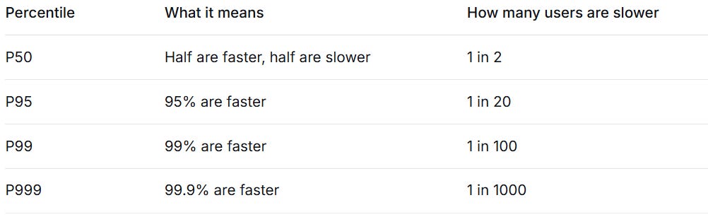
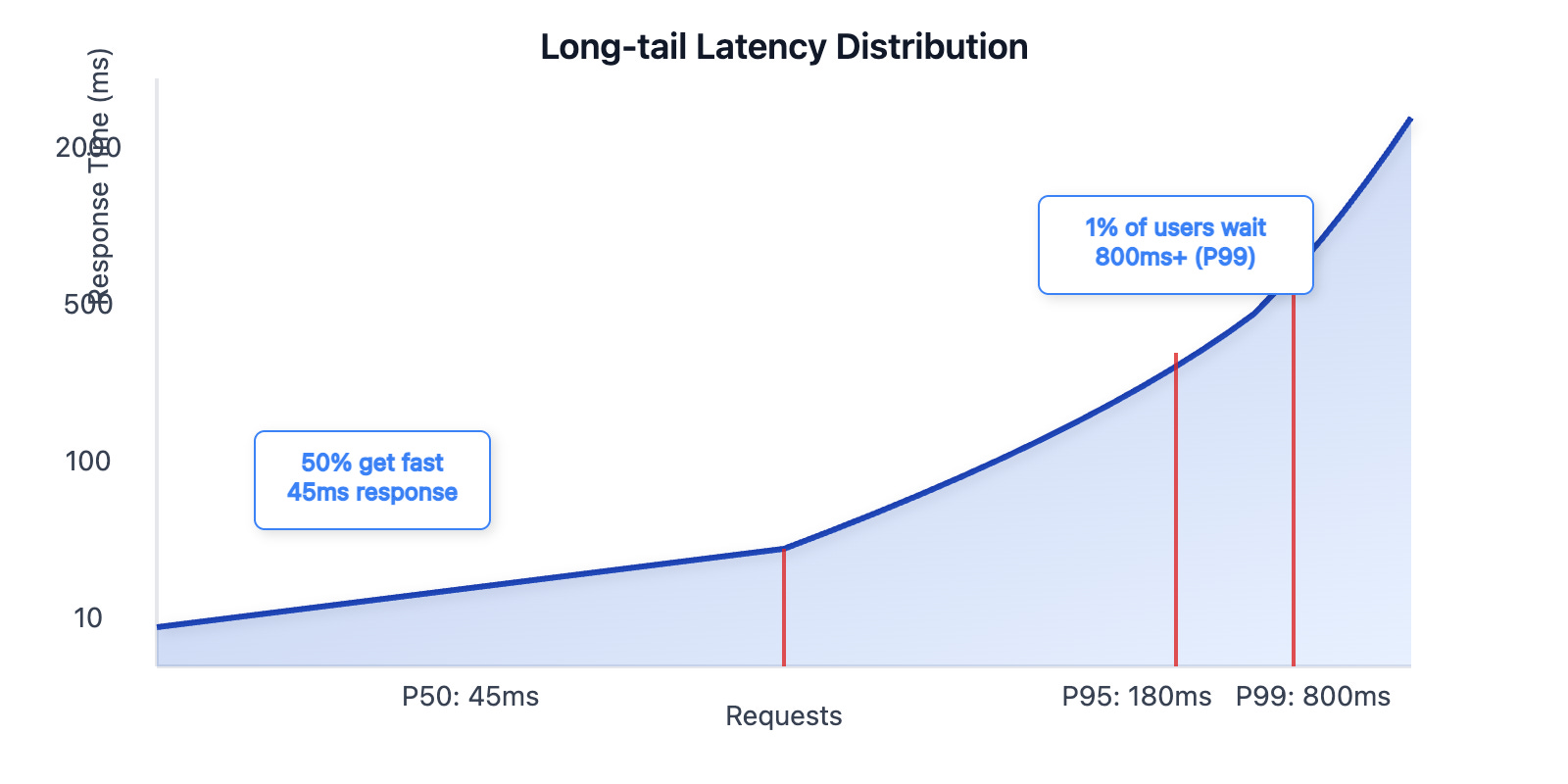
P50 (the median): 50% of requests are faster than this. 50% are slower. Half your users experience latency below P50. Half experience latency above P50.
P95: 95% of requests are faster than this. 5% of requests are slower. One out of every twenty users experiences latency above P95.
P99: 99% of requests are faster than this. 1% of requests are slower. One out of every hundred users experiences latency above P99.
P999: 99.9% of requests are faster than this. 0.1% of requests are slower. One out of every thousand users experiences latency above P999.
The Same Example with Percentiles
The same 100 requests: 99 at 10ms, 1 at 10,000ms.
Average: 110ms (misleadingly good)
P50: 10ms (half of requests are 10ms or faster)
P95: 10ms (95% of requests are 10ms or faster)
P99: 10,000ms (99% of requests are 10,000ms or faster)
P99 tells the truth. One percent of requests take ten seconds. That is the number that matters.
Visualized graph with different numbers but same concept
Tail Latency
Tail latency means the high percentiles: P99, P999, and beyond. These represent the slowest requests, the ones at the far end of the distribution.
Why does tail latency matter more in distributed systems than in single services?
Imagine one request fans out to 100 different services in parallel. Each service has P99 = 100ms. That means each service has a 1% chance of being slower than 100ms.
The chance that all 100 services are faster than 100ms is:
text
0.99 ^ 100 ≈ 0.37That is 37%. The chance that at least one service is slower than 100ms is 63%.
Even though each individual service is fast 99% of the time, the overall request experiences tail latency 63% of the time. Tail latency multiplies.
So which measure to use for what?
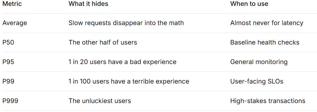
Average latency tells you about the center of your distribution. But users do not experience the center. Each user experiences a single request. If that request is slow, the system is slow for that user. Percentiles measure what users actually feel.